Introduction

Public expenditure aims at improving the well-being of people through the provision of efficient public services, and at the same time, it also works as a crucial determinant of economic growth, especially in developing countries. Public expenditure incurred on the expansion of infrastructure facilities like telecommunication, power, roads and railways, etc., positively affects economic growth (Singh, 2022). It is argued that public expenditure on health services, education facilities, social welfare and cultural activities, etc., reflects in growth as well as productivity of a country, albeit with some time lag owing to its distributive nature (Marjit et al., 2020). Moreover, public expenditure accelerates economic growth through the channel of human capital formed with the help of adequate infrastructure pertaining to schooling and skill formation (Agenor, 2008).

The analysis of the relationship between public expenditure and economic growth gained substantial consideration in the academic circles as well as public policy discourses in both the developed and developing countries (Barro, 1990; Chletsos & Kollias, 1997; Jones & Sunday, 2016; Landau, 1983; Peacock & Scott, 2000). The existing body of literature furnished distinctive theoretical arguments and empirical evidence about the public expenditure-economic growth nexus (Ahuja & Pandit, 2020; Ray et al., 2019). As a result, two opposing theories of public expenditure, namely, Wagner’s law (1958) and Keynes’s hypothesis (1936), emerged in the vast economics and public finance literature, both supporting the public expenditure-economic growth nexus. However, Wagner’s law, widely accepted in public finance, viewed public expenditure as an endogenous factor which is caused by economic growth (Henrekson, 1993; Jones & Sunday, 2016), whereas Keynesian hypothesis, popular in the field of economics, regarded public expenditure as an exogenous factor and vital policy instrument to stimulate economic growth (Ansari et al., 1997; Ray et al., 2019).

The composition as well as productivity of various components of public expenditure also have a bearing on economic growth. Various studies aimed at investigating the effects of the composition of public expenditure on economic growth have produced mixed results (Agenor, 2008; Barro, 1990; Devarajan et al., 1996; Marjit et al., 2020). Capital component of public expenditure is regarded as a cornerstone of economic development and a pivotal catalyst to spur economic growth by enhancing the level of physical capital, which further yields propitious growth effects (Mohapatra & Mishra, 2011). It is argued that the benefits of capital expenditure (CE) accrue after some time lag, and it also complements the positive gains stemming from the revenue component of public expenditure. Devarajan et al. (1996) observed that an increase in the share of current expenditure positively and significantly affects economic growth, while the capital component of public expenditure exudes a negative relationship with economic growth. Marjit et al. (2020) found that the capital component of public expenditure has a positive and significant impact on economic growth, whereas the revenue component of public expenditure demonstrated a negative effect on economic growth in the Indian context.

Policymakers and scholars are divided on the question of whether public expenditure spurs or hinders economic growth due to the conflicting results produced by various studies focused on analysing the linkages between public expenditure and economic growth. Advocates of bigger governments argued that an increase in public expenditure, especially on socio-economic and physical infrastructure facilities, contributes positively to enhancing economic growth (Akpan & Abang, 2013). However, proponents of smaller governments pointed out that higher public expenditure can stifle economic growth (Landau, 1983). Moreover, it is posited that low-income countries characterised by poor institutions and rampant corruption normally cause public expenditure to be irrelevant or destructive to economic growth (Wu et al., 2010). Several researchers, while distinguishing between productive and unproductive heads of public expenditure, highlighted that not all public spending is growth-stimulating (Devarajan et al., 1996).

Another unpopular strand called ‘neutrality view’ exhibits that public expenditure and economic growth are independent of each other and do not cause each other (Ansari et al., 1997). However, a negative and statistically significant effect of public expenditure on economic growth has also been observed (Barro & Sala-i-Martin, 1995). The divergent evidence and views about the relationship between public expenditure and economic growth make its analysis more imperative and relevant for a developing country like India, which has witnessed increased levels of government spending over the years. The growing government spending tends to be associated with increasing fiscal deficit and indicates a limited ability to raise sufficient funds to finance escalating public expenditure on the part of governments. With this backdrop, the present study attempts to investigate the relationship between public expenditure and economic growth in India.

The article is divided into six sections. Section 1 provides the introduction, whereas Section 2 sheds light on some stylised facts about public expenditure in India. Section 3 outlines the literature review, and Section 4 elucidates the materials and methods used in the study. Section 5 contains the results and discussion, while the conclusion of the study is presented in Section 6.

Public Expenditure in India: Some Stylised Facts

There is no paucity of trials and tribulations when it comes to the question of growth and development for a developing country like India (Ray et al., 2019; Singh, 2024). After gaining independence, the arduous challenges of poverty reduction, infrastructure development, employment generation, economic development, as well as enhancement in the well-being of the public lay before the Government of India. In line with these onerous tasks, public expenditure has been incurred on social services, including education and health, economic services, and various other categories in order to improve the level of human development and keep up with the rapidly advancing world (Marjit et al., 2020; Mohapatra & Mishra, 2011; Singh, 2025a).

Figure 1 presents the trend in the combined public expenditure of the Centre and State Governments in India. Figure 1 shows that both series, that is, combined revenue expenditure (RE) and combined CE, follow an overall upward trajectory across the entire period, indicating that the role of government expenditure in the economy has expanded significantly over time. However, the increase is not uniform; rather, it occurs in phases, with some periods showing slow growth and others showing much sharper acceleration.

 

Figure 1. Centre and State Governments’ Combined Public Expenditure in India (% of GDP), 1970–1971 to 2024–2025.

 

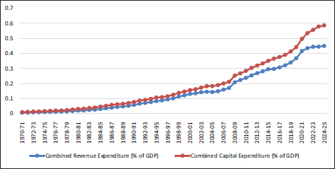
In the earlier decades, from the 1970s through the mid-1990s, both revenue and CE remained at relatively low levels as a share of gross domestic product (GDP), though they rose gradually. This suggests that public spending was expanding, but in a measured and incremental manner. The close movement of the two lines during this phase indicates that both forms of expenditure were increasing together without a large divergence. The gradual rise may be associated with the expansion of government responsibilities in areas such as administration, public services, infrastructure, and development programmes, but the overall fiscal size of the state remained moderate relative to later years. The relatively flatter slope of the lines in this period reflects limited acceleration in public expenditure intensity.

From around the late 1990s to the late 2000s, public expenditure began to exhibit a stronger upward movement. Both revenue and CE increase more visibly, reflecting a structural change in the expenditure pattern. RE rises steadily, which may indicate growing commitments toward salaries, subsidies, grants, interest payments, welfare schemes, and other recurring obligations. CE also rises at a faster pace, remaining consistently above RE in the chart. This is significant because CE is generally associated with long-term asset creation, such as roads, irrigation works, public buildings, transport systems, and other developmental infrastructure. The higher position of the CE line implies that the growth in public investment has been comparatively stronger, which may be interpreted as a positive sign for development-oriented fiscal policy.

After 2009–2010, both series display a marked and sustained increase. The RE line rises sharply, but the CE line rises even more steeply, especially after 2020–2021. In 2024–2025, CE reaches nearly 0.58%–0.59% of GDP, while RE climbs to about 0.45%–0.46% of GDP. This widening gap between the two lines indicates that capital spending has grown more rapidly than revenue spending in recent years. Such a pattern may be justified by the increasing policy emphasis on infrastructure-led growth, economic recovery measures, and public investment as a tool for stimulating output, employment, and private sector confidence. The sharper post-2020 rise may also reflect extraordinary fiscal interventions and renewed emphasis on capital formation in response to economic disruptions and development needs.

Public expenditure by the centre and states together has increased substantially over time, indicating a larger fiscal role of government in the Indian economy. Although both revenue and CE have grown, CE has remained consistently higher and has accelerated more sharply in the recent period, suggesting a stronger developmental and investment orientation in fiscal policy. The recent steep rise in both components demonstrates that government spending has become an increasingly important instrument for supporting growth, providing public services, and building economic capacity. This not only suggests the quantitative expansion of public expenditure but also reflects an important qualitative shift toward higher capital outlay, which has stronger long-term implications for economic development and structural transformation.

Literature Review

Various studies assessing the relationship between public expenditure and economic growth, both in terms of theoretical investigation and empirical analysis, can be traced in the extant literature. These studies mainly intended to test the validity of either Wagner’s law or Keynesian hypothesis of public expenditure. The first group of studies devoted to testing the validity of Wagner’s law of public expenditure found evidence in support of Wagner’s law (Chang, 2002; Chletsos & Kollias, 1997; Mohsin et al., 1992; Thornton, 1999). Singh (1997) investigated the causality between public expenditure and per capita gross national product employing regression analysis. The study found that Wagner’s law of public expenditure is valid in the context of the Indian economy. Chang (2002) tested the validity of Wagner’s law in six countries, namely South Korea, Taiwan, Thailand, Japan, the USA and the United Kingdom by utilising annual time series data between 1951 and 1996. The results indicated that there was unidirectional causality running from income to public expenditure in selected countries, with the exception of Thailand.

Basu and Datta (2009) examined the relationship between public expenditure and economic growth using Granger’s causality test. The findings of the study supported Wagner’s law, that is, economic growth leads to public expenditure in India. Grullon (2012) analysed the causal link between national income and government spending during 1960–1984 and 1985–2005, applying the bounds testing approach and the Granger pairwise causality test. The study found that there is evidence of causality from GDP to government spending and confirmed the validity of Wagner’s law in the case of the Dominican Republic.

Another set of studies pertaining to the analysis of public expenditure and economic growth presented empirical evidence in support of the Keynesian theory of public expenditure (Chen, 2006; Ebaidalla, 2013; Kotosz, 2006; Lin, 1994; Yasin, 2003). Ghali (1998) assessed the impact of public expenditure on economic growth in 10 OECD countries using quarterly data for 1970–1994. The findings of the study supported the Keynesian hypothesis, that is, public expenditure directly as well as indirectly Granger-causes economic growth in the selected countries. Jiranyakul and Brahmasrene (2007) examined the causal link between public expenditure and economic growth in Thailand, applying the Granger causality test. The results concluded that there exists unidirectional causality running from public expenditure to economic growth. Cosimo (2010) investigated the association of public expenditure and economic growth in Italy using time series data for 1960–2008. It was found that public expenditure positively influences economic growth in Italy.

Gemmell et al. (2016) evaluated the impact of size and composition of public expenditure on GDP per capita in OECD countries. The findings of the study revealed that public expenditure on education, housing, health, and transport and communication positively affect per capita GDP in the long-run. Ahuja and Pandit (2020) inspected the relationship between public expenditure and economic growth in 59 countries using panel data for the time period of 1990–2019. The findings of the study supported the Keynesian hypothesis that asserts the significance of public expenditure in boosting economic growth. Moreover, the Keynesian framework advocating the significance of government expenditure in accelerating national economies has been widely adopted in developing countries due to various factors such as market failures, and the private sector’s inability to provide public goods as a result of capitalist behaviour and monopolistic tendencies (Jones & Sunday, 2016).

Apart from the above-reviewed two groups of studies, there are some research endeavours which yielded mixed results pertaining to the issue of the public expenditure-economic growth nexus. A few studies also supported the feedback relationship between public expenditure and economic growth. Mohsin et al. (1992) and Singh and Sahni (1984) suggested the presence of bi-directional causality between public expenditure and economic growth in India. In some cases, the negative impact of public expenditure on economic growth in both developing and developed countries has also been detected (Diamond, 1989; Mitra, 2006). Moreover, Kormendi and Meguire (1985) and Maku and Ajike (2014) reported that there is no causal link between public expenditure and economic growth.

Some researchers argued that Wagner’s law of ‘increasing public and state activities’ is a long-run phenomenon (Henrekson, 1993), and there is no co-movement between public expenditure and economic growth in the short run (Ahsan et al., 1996). Moreover, Wagner’s law implied regularities or empirically observed uniformity in the pattern of growth of government expenditure and economic growth, and it does not necessarily imply causation between the two variables under consideration (Peacock & Scott, 2000). However, it is pointed out that the existence of a long-run relationship indicates the prevalence of inter-temporal association accentuated by a prima facie causative process between public expenditure and economic growth in the short-run (Ansari et al., 1997; Narayan et al., 2008).

The precise information regarding the direction of causality between public expenditure and economic growth is of paramount significance in order to adopt effective policy measures. Empirical evidence of a causal flow consistent with Wagner’s law considers public expenditure as a passive factor, whereas the causative process validating the Keynesian hypothesis views public expenditure as a critical policy instrument to promote economic growth. Moreover, the analysis of the relationship between public expenditure and economic growth is vital from the perspective of public finance sustainability, as governments are struggling to restrain public spending, especially in developing countries like India. Keeping this in mind, this article seeks to investigate the causal relationship between public expenditure and economic growth in India.

Materials and Methods

Data

This study analyses the relationship between public expenditure and economic growth in India from 1970–1971 to 2024–2025. The data are sourced from the Handbook of Statistics on the Indian Economy published by the Reserve Bank of India (2026). Public expenditure is bifurcated into two components, that is, CE of both central government and state governments as a percentage of GDP (CE), and RE of both central government and state governments as a percentage of GDP (RE). The data pertaining to GDP per capita is used as a proxy for economic growth. The data for GDP per capita is transformed into a natural logarithm (lnGDP).

Unit Root Tests

The time series data pertaining to the macroeconomic variables contains unit roots dominated by stochastic trends. The non-stationary time series possess time-varying mean or variance or both, and the presence of non-stationary regressors can yield spurious results (Gujarati et al., 2012). Therefore, one of the fundamental steps in time series analysis is to test the stationarity of the variables (Singh, 2025b). In the present study, unit root tests were conducted employing the Augmented-Dickey-Fuller (ADF) test (Dickey & Fuller, 1979) and the Phillips-Perron (PP) test (Phillips & Perron, 1988). The ADF test and PP test entail the estimation of the regression equations as given by Equations (1) and (2), respectively.

                    (1)

 

          (2) 

Where,

  = First difference of Y_t

  = Constant

  =   -1

 m = Lag length

  = White noise error term.

Cointegration Test

After confirming the presence of a unit root in the data series, the next step was to examine whether a long-run equilibrium relationship exists among the variables under consideration. Variables are considered cointegrated when they are individually non-stationary at the level, but a linear combination of these integrated variables is stationary (Enders, 2010). In order to investigate the long-run relationship between public expenditure and economic growth, the Johansen cointegration test, as given by Equation (3) (Johansen, 1988), is applied.

                                                 (3)

The number of cointegrated vectors was tested using the trace statistic and the maximum eigenvalue statistic. The trace statistic and the maximum eigenvalue statistic are constructed as given by Equations (4) and (5), respectively.

                                               (4) 

 

                                          (5) 

Where,

 = The estimated value of the characteristic root derived from the calculated matrix.

r = Number of cointegrating vectors under the null hypothesis.

T = Number of usable observations.

ln = Natural logarithm.

The trace statistic tested the null hypothesis that the number of cointegrating vectors was less than or equal to r against the alternative hypothesis of more than r cointegrating vectors. The maximum eigenvalue statistic tested the null hypothesis that the number of cointegrating vectors was equal to r against the alternative hypothesis of r + 1 cointegrating vectors (Enders, 2010). A significant non-zero eigenvalue represented a significant number of cointegrating vectors. The Johansen cointegration test was widely used in the existing literature to explore the relationship between different variables (Akpan & Abang, 2013; Mohapatra & Mishra, 2011; Ramphul, 2012). The justification for using Johansen cointegration test lies in the fact that this test helps in reducing the spurious rejection frequency when the analysis is based on a limited number of variables (Hjalmarsson & Osterholm, 2010). Moreover, this test was used in the present analysis due to its ability to detect cointegration among variables that are integrated of order one, I(1), that is, non-stationary in levels but stationary in first differences (Shrestha & Bhatta, 2018).

Testing for Causality

If public expenditure and economic growth are cointegrated, then causality must exist in at least one direction. To assess the direction of causality between public expenditure and economic growth, the Granger causality test based on the bivariate regression model as given by Equations (6) and (7) (Granger, 1986) is used.

                                  (6) 

 

                          (7) 

There will be unidirectional causality running from X to Y if the set of lagged X coefficients computed in Equation (6) is statistically different from zero as a group, while the set of calculated coefficients on lagged values of Y is not statistically different from zero. In case of unidirectional causality running from Y to X, the estimated coefficients on lagged values of Y in Equation (7) will be statistically different from zero and the measured coefficients on lagged values of X will not be statistically different from zero (Gujarati et al., 2012). Several studies have applied the Johansen cointegration test and Granger causality test to analyse the relationship between different variables (Akpan & Abang, 2013; Mohapatra & Mishra, 2011; Ramphul, 2012). The present study used the same framework employed by these studies.

Results and Discussion

Table 1 presents the descriptive statistics of the variables used in the study. The mean values of CE (11.43), RE (12.58), and lnGDP (10.62) were closer to their respective medians, indicating a balanced distribution of the data. The range between maximum and minimum values revealed that RE had higher variation compared to CE and lnGDP. The standard deviation further confirmed this, as RE (2.13) showed higher variability, while lnGDP (0.59) remained stable over the study period. The skewness values divulged that CE was almost symmetric, RE was slightly negatively skewed, and lnGDP was moderately positively skewed. The kurtosis values for all variables were below 3, suggesting platykurtic distributions with fewer extreme observations. The Jarque-Bera test probabilities for CE (0.2956), RE (0.1821), and lnGDP (0.1003) were all greater than 0.05, implying that the null hypothesis of normality could not be rejected, and therefore the variables were normally distributed.

 

Table 1. Descriptive Statistics of Variables.

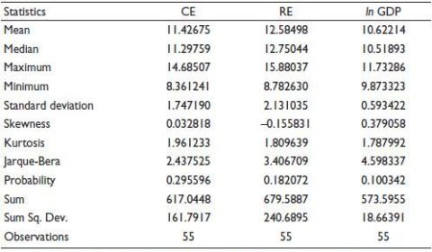
Note: CE: Capital expenditure of both central government and state governments as percentage of GDP, RE: Revenue expenditure of both central government and state governments as percentage of GDP, lnGDP: Natural logarithm of GDP.

 

The time series properties of the variables were tested for stationarity using the unit root tests. ADF test and PP test were employed to test the unit root of the data. The results of the ADF and PP unit root tests were presented in Table 2. The null hypothesis of non-stationarity of CE, RE and GDP per capita (lnGDP) was tested against the alternative hypothesis of stationarity of these variables. The results revealed that CE was non-stationary at the level with intercept as well as with intercept and trend. It indicated the presence of a unit root in the data series. The results showed that RE was stationary at a level with intercept, but it was non-stationary at a level with intercept and trend.

 

Table 2. Unit Root Tests.

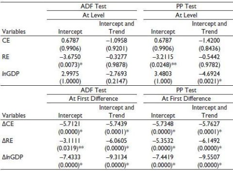
Notes: ADF: Augmented Dickey-Fuller, PP: Phillips-Perron. Values in parentheses are p values. * and ** denote the statistical significance at 1% and 5% levels, respectively. Δ represents the first difference of the series; ln indicates that the variable is transformed into natural logarithms.

 

Further, the results of the ADF test exhibited that GDP per capita was non-stationary at the level with intercept as well as with intercept and trend. However, the results of the PP test showed that GDP per capita was non-stationary at the level with intercept, but it was stationary at the level with intercept and trend. The results confirmed that CE, RE and GDP per capita were stationary at first difference with intercept and trend, that is, there was evidence supporting the absence of a unit root. Since all of the variables were integrated of order one, that is, I(1), there was a possibility that these data series might be cointegrated.

After conducting the ADF and PP unit root tests, Johansen’s cointegration test was performed to examine the long-run relationship between public expenditure and economic growth. The results of the Johansen test for cointegration were reported in Table 3. The test rejected the null hypothesis of no cointegration at 5% significance level, and it was concluded that public expenditure and economic growth were cointegrated, that is, they co-moved in the long run. The number of cointegrating relationships among the underlying variables was tested using the trace statistic and the maximum eigenvalue statistic. The results of both trace and maximum eigenvalue rank tests revealed that cointegration existed among the set of variables at 5% level of significance. The trace statistic, as well as the maximum eigenvalue statistics, identified two cointegrating vectors. The results of the trace test and maximum eigenvalue test suggested a cointegrating equation among variables at 5% significance level. As the variables were cointegrated, the corresponding cointegrating equation was described as given by Equation (8).

                                                    

                                                      (8)

 

Table 3. Johansen Test for Cointegration.

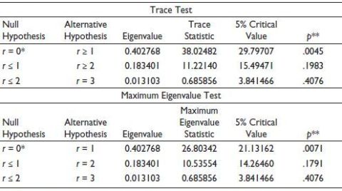
Notes: ‘r’ indicates the number of cointegrating vectors. *represents rejection of the null hypothesis at the 5% significance level. **denotes MacKinnon et al. (1999) p values.

 

In Equation (8), the estimated cointegrating vector was normalised with respect to lnGDP by setting its coefficients equal to 1, enabling a straightforward reading of different elasticities. The numbers in parentheses were asymptotic standard errors. The equation revealed that the presence of a negative relationship between CE and economic growth in the long-run. However, RE exerted a positive influence on economic growth in the long-run. Therefore, the results supported the proposition that there existed a stable long-run relationship between public expenditure and economic growth in India. It was pertinent to assert that variables were moving together, and they did not tend to move far from each other in the long-run. However, without evidence of causality, it was difficult to state whether Wagner’s law or Keynesian hypothesis was valid in the case of India.

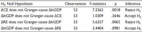
The Granger causality test was conducted to ascertain the direction of causality between public expenditure and economic growth. The results of the Granger causality test were presented in Table 4. The results suggested that both CE and RE had a causal effect on economic growth. Further, it was revealed that there was no effect of economic growth on CE as well as RE. Thereby, the results confirmed the validity of the Keynesian hypothesis in India, whereas the results refuted the presence of Wagner’s law in India. The findings of the study were consistent with the results of Ramphul (2012), Ebaidalla (2013), Kotosz (2006) and Ahuja and Pandit (2020), who supported the existence of the Keynesian hypothesis, that is, public expenditure promoted economic growth. The results of the present study were also in tandem with the findings of Ramphul (2012) and Sagarik (2016), who refuted the existence of Wagner’s law. However, the results of the present study were in contrast with the findings of Singh (1997) and Basu and Datta (2009), who reported that economic growth stimulated public expenditure. Thereby, they had supported the existence of Wagner’s law.

 

Table 4. Granger Causality Test.

 

CE was regarded as a cornerstone of economic development and a pivotal catalyst to spur economic growth in a country by enhancing the level of physical capital, which further yielded propitious growth effects (Mohapatra & Mishra, 2011). CE included infrastructure development, that is, roads, bridges, parks, stadiums, industrial and commercial zones, etc., which boosted economic growth by directly increasing the national output (Paudel, 2023). It was also associated with other growth-promoting attributes like strong employment generation potential as well as backward and forward linkages with other sectors of the economy (RBI, 2022). A higher share of CE in public expenditure was strongly associated with greater public infrastructure investments, better education and health care services, as well as improved research and development that support growth by ameliorating the endowment as well as productivity of factors of production (Chu et al., 1995; Leoni, 2025). Moreover, it was argued that the benefits of CE accrued after some lag, complementing the positive gains stemming from RE.

The state incurred public expenditure to achieve sustainable and equitable economic growth. The higher proportion of RE indicated that the management of government spending needs to be revamped, as the recent exponential growth witnessed in it was not sustainable and called for its restraint as well as rationalisation. Juxtaposing this rampant growth of RE with the plummeting growth in CE, it appeared that not only were the gains from economic growth being insufficiently used for infrastructure development and asset creation, but also the minuscule amount of CE accrued by the government was being hindered by low productivity and inefficient resource use.

Even though the role of the state in the Indian economy had declined in the post-reform period, it still remained a prominent economic agent providing momentum and stability to the economy, steering it in the right direction with public expenditure as a foremost aid at its disposal. Certain components of RE, such as payment of wages and defence expenditure, formed an important part and were inevitable. However, the components such as expenditure on subsidies and interest payments, etc., offered scope for their rationalisation and reallocation so that these funds could be appropriately used for asset creation. A prudent expenditure management was the way to go to buckle up for challenges and maintain a balance between the RE and CE to make it more productive.

Conclusion

Public expenditure is seen as a central facilitator of economic growth through physical and human capital formation achieved using expenditure on expansion of infrastructural facilities like power, roads and railways, etc., and provision of education, health and other such social services, whereby different components of public expenditure have been observed to produce varied growth effects. Simultaneously, the stifling effects of public expenditure on economic growth have also been observed, especially in low-income countries, rampant with poor institutions and widespread corruption, rendering it irrelevant and destructive.

The present study investigates the causal relationship between public expenditure and economic growth in India during 1970–1971 to 2024–2025. The cointegration test confirms that public expenditure and economic growth were cointegrated in the long-run. This indicates that there exists a stable long-run relationship between public expenditure and economic growth in India. The Granger causality test shows a unidirectional causality running from public expenditure (both RE and CE) to economic growth, which supports the Keynesian hypothesis in the case of India. However, it is observed that economic growth has no causal effect on CE and RE.

The results suggest that the Keynesian hypothesis, that is, public expenditure causes economic growth, is valid in the case of India, while Wagner’s laws, that is, public expenditure is caused by economic growth, stand invalid in India. The results indicate that the existing framework of public expenditure has been fruitful in terms of encouraging economic growth in India. The importance of CE in alleviating the endowment as well as productivity of factors of production, accompanied by its catalytic linkages with other sectors of the economy, cannot be disregarded, as it may prove inimical to the growth prospects of the economy. Moreover, RE contributes to economic growth through various channels, such as human capital development and consumer demand. The study recommends that policymakers should adopt an expansionary yet well-structured fiscal strategy that prioritises productive public expenditure. A balanced expansion of both capital and RE, combined with improved fiscal governance and efficient allocation of public funds, can serve as an effective policy tool for boosting long-term economic growth in India.

Declaration of Conflicting Interests

The authors declared no potential conflicts of interest with respect to the research, authorship and/or publication of this article.

Funding

The authors received no financial support for the research, authorship and/or publication of this article.

ORCID iDs

Kulwinder Singh  https://orcid.org/0000-0001-6620-598X

Jagmohan Singh  https://orcid.org/0000-0002-6873-4188

Anish Slath  https://orcid.org/0000-0002-0350-3565